Portfolio

Portfolio continuation

New inv2026.9.5

✅ Pick up right where your simulation left off as new data arrives. VBT carries positions, order IDs, and stop state into each update, including entry timestamps and trailing highs. Your trailing stops remember their peaks, your time stops keep counting, and each update returns a new portfolio with the combined history.

Preserve a trailing stop across two updates

close = pd.Series(
    [100.0, 110.0, 108.0, 98.0, 103.0, 115.0],
    index=pd.date_range("2026-09-01", periods=6, freq="D")
)
entries = pd.Series([True, False, False, False, True, False], index=close.index)
pf_kwargs = dict(size=1, init_cash=1000, tsl_stop=0.05, freq="1D")

pf = vbt.PF.from_signals(
    close.iloc[:2],
    entries=entries.iloc[:2],
    attach_preparer=True,  
    **pf_kwargs,
)
for start in [2, 4]:
    pf = pf.update(  
        close.iloc[start:start + 2],
        entries=entries.iloc[start:start + 2],
    )

print(pf.orders.readable[["Order Id", "Fill Index", "Side", "Price", "Stop Type"]])

   Order Id Fill Index  Side  Price Stop Type
0         0 2026-09-01   Buy  100.0      None
1         1 2026-09-04  Sell   98.0       TSL
2         2 2026-09-05   Buy  103.0      None

full_pf = vbt.PF.from_signals(close, entries=entries, **pf_kwargs)  
pf.orders.records.equals(full_pf.orders.records) and pf.value.equals(full_pf.value)

True

Tutorial

Learn more in the Live simulation tutorial.

Portfolio from fills

New inv2026.9.5

✅ Turn your execution records into a VBT portfolio and explore trades, drawdowns, and performance with the same tools you use for backtests. Missing record fields receive defaults, and readable side names are mapped automatically, keeping the setup light.

Calculate portfolio value and profit from two fills

close = pd.Series(
    [100.0, 105.0, 110.0],
    index=pd.date_range("2026-09-01", periods=3, freq="D")
)
fills = [
    dict(idx=0, size=2, price=100, fees=1, side="Buy"),
    dict(idx=2, size=2, price=110, fees=1, side="Sell"),
]
pf = vbt.PF(close, order_records=fills, init_cash=1000, freq="1D")

print(pf.total_profit)

18.0

pf.value.tolist()

[999.0, 1009.0, 1018.0]

Contract multiplier

New inv2026.4.7

✅ All simulation entry points now accept a multiplier that scales every order by a constant factor, making it straightforward to model futures contracts and other derivatives where one contract represents multiple units of the underlying asset.

SMA crossover on E-mini S&P 500 futures

data = vbt.YFData.pull("ES=F", start="2023", end="2024")  

fast_sma = data.run("talib_func:sma", timeperiod=10)  
slow_sma = data.run("talib_func:sma", timeperiod=30)
entries = fast_sma.vbt.crossed_above(slow_sma)
exits = fast_sma.vbt.crossed_below(slow_sma)

pf_stock = vbt.PF.from_signals(  
    data,
    entries=entries,
    exits=exits,
    size=1,
    init_cash=500_000,
)

pf_futures = vbt.PF.from_signals(  
    data,
    entries=entries,
    exits=exits,
    size=1,
    multiplier=50,
    init_cash=500_000,
)

print(pf_stock.total_profit)

627.25

print(pf_futures.total_profit)

31362.5

print(pf_futures.trades.readable[["Avg Entry Price", "Avg Exit Price", "PnL", "Return"]])

   Avg Entry Price  Avg Exit Price      PnL    Return
0          4057.50         4138.00   4025.0  0.019840
1          4212.00         4480.75  13437.5  0.063806
2          4490.25         4378.75  -5575.0 -0.024832
3          4430.50         4820.00  19475.0  0.087913

Negative price

New inv2026.4.7

✅ The simulation engine previously rejected negative prices at validation time, making it impossible to model instruments whose price can legally go below zero (such as the infamous April 2020 WTI crude oil event). Negative prices are now fully supported across the entire pipeline.

Long WTI crude oil through the April 2020

data = vbt.YFData.pull("CL=F", start="2020-02-01", end="2020-07-01")  

entries = pd.Series(False, index=data.index)  
exits = pd.Series(False, index=data.index)
entries["2020-03-03"] = True
exits["2020-05-04"] = True

pf = vbt.PF.from_signals(  
    data,
    entries=entries,
    exits=exits,
    size=1,
    multiplier=1000,
    init_cash=200_000,
)

print(data.close[data.close < 0])

Date
2020-04-20 00:00:00-04:00   -37.630001
Name: Close, dtype: float64

print(pf.trades.readable[["Avg Entry Price", "Avg Exit Price", "PnL", "Return"]])

   Avg Entry Price  Avg Exit Price           PnL    Return
0            47.18       20.389999 -26790.000916 -0.567825

print(pf.value[["2020-03-03", "2020-03-09", "2020-04-20", "2020-05-04"]].round(2))

Date
2020-03-03 00:00:00-05:00    200000.0
2020-03-09 00:00:00-04:00    183950.0
2020-04-20 00:00:00-04:00    115190.0
2020-05-04 00:00:00-04:00    173210.0
Name: value, dtype: float64

Chaining simulations

New inv2026.3.1

✅ Every built-in simulation function now returns the final simulation state after processing all data, including the last cash, position, pending order(s), and other relevant information. This state can be passed to the next simulation run, allowing you to continue from where the previous run ended. This enables seamless chaining of simulations across different time periods or datasets.

Simulate a SMA crossover strategy on a monthly basis

data = vbt.BinanceData.pull(  
    "BTCUSDT",
    start="one year ago",
    timeframe="5 minutes",
    cache=True
)

fast_sma = data.run("talib_func:sma", timeperiod=20)  
slow_sma = data.run("talib_func:sma", timeperiod=50)
long_entries = fast_sma.vbt.crossed_above(slow_sma)
short_entries = fast_sma.vbt.crossed_below(slow_sma)

single_pf = vbt.PF.from_signals(  
    data,
    long_entries=long_entries,
    short_entries=short_entries,
)

data_splits = data.split(by="month")  
long_entries_splits = long_entries.vbt.split(by="month", into=None)
short_entries_splits = short_entries.vbt.split(by="month", into=None)

pf_list = []
last_state = None
for i in range(len(data_splits)):  
    pf = vbt.PF.from_signals(
        data_splits.iloc[i],
        long_entries=long_entries_splits.iloc[i],
        short_entries=short_entries_splits.iloc[i],
        last_state=last_state,
    )
    pf_list.append(pf)
    last_state = pf.last_state

stacked_pf = vbt.PF.row_stack(*pf_list, chained=True)  
print(stacked_pf.returns.equals(single_pf.returns))

True

Full callback support

New inv2025.12.31

✅ Portfolio simulation method based on signals now fully supports callbacks at every step of the process. This includes pre-processing and post-processing callbacks for the simulation as a whole, as well as per-group and per-segment callbacks, and even an order modification callback. This allows you to customize the simulation behavior to a great extent.

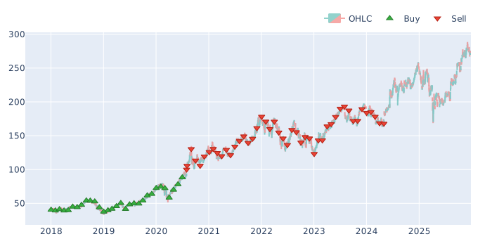
DCA in $100 every month until 2x in profit, take out initial investment, and DCA out

DCAMode = namedtuple("DCAMode", ["In", "Out"])(0, 1)  

@njit
def pre_group_func_nb(ctx):  
    total_deposited = np.full(1, 0.0)
    dca_mode = np.full(1, DCAMode.In)
    return (total_deposited, dca_mode)

@njit
def pre_segment_func_nb(ctx, total_deposited, dca_mode, cash_deposits, dca_amount):  
    if ctx.i == 0 or vbt.dt_nb.month_nb(ctx.index[ctx.i - 1]) != vbt.dt_nb.month_nb(ctx.index[ctx.i]):
        dca_amount_now = vbt.pf_nb.select_from_group_nb(ctx, ctx.group, dca_amount)
        if dca_mode[0] == DCAMode.In and ctx.track_cash_deposits:
            cash_deposits[ctx.i, ctx.group] = dca_amount_now
            total_deposited[0] += dca_amount_now
    else:
        dca_amount_now = 0.0
    return (total_deposited, dca_mode, dca_amount_now)

@njit
def signal_func_nb(ctx, total_deposited, dca_mode, dca_amount_now, size):  
    if dca_amount_now > 0:
        size[ctx.i, ctx.col] = dca_amount_now
        if dca_mode[0] == DCAMode.In:
            return True, False, False, False
        return False, True, False, False
    return False, False, False, False

@njit
def post_order_func_nb(ctx, total_deposited, dca_mode, dca_amount_now):  
    if dca_mode[0] == DCAMode.In:
        if vbt.pf_nb.order_increased_position_nb(ctx):
            tp_info = ctx.last_tp_info[ctx.col]
            tp_info["stop"] = 1.0
            tp_info["init_price"] = ctx.last_pos_info[ctx.col]["entry_price"]
            tp_info["exit_size"] = total_deposited[0]
            tp_info["exit_size_type"] = vbt.pf_enums.SizeType.Value
        elif vbt.pf_nb.get_last_order_nb(ctx)["stop_type"] == vbt.pf_enums.StopType.TP:
            dca_mode[0] = DCAMode.Out

pf = vbt.PF.from_signals(
    vbt.YFData.pull("AAPL", start="2018"),
    pre_group_func_nb=pre_group_func_nb,
    pre_segment_func_nb=pre_segment_func_nb,
    pre_segment_args=(
        vbt.Rep("cash_deposits"),
        vbt.Rep("dca_amount")
    ),
    signal_func_nb=signal_func_nb,
    signal_args=(
        vbt.Rep("size"),
    ),
    post_order_func_nb=post_order_func_nb,
    broadcast_named_args=dict(dca_amount=100),
    arg_config=dict(
        cash_deposits=dict(full_shape=True),  
        size=dict(full_shape=True)
    ),
    accumulate=True,
    size_type="value",
    cash_sharing=True
)
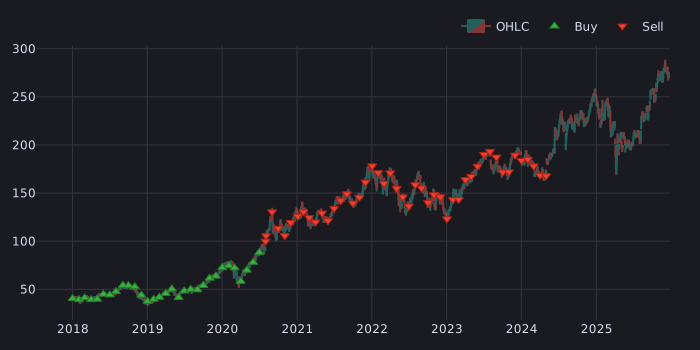
pf.plot_orders().show()

Documentation

Learn more in the Documentation → Portfolio → From signals → Callbacks.

Asset weighting

New inv2024.8.20

✅ Asset weighting lets you fine-tune the influence of individual assets or strategies within your portfolio, giving you enhanced control over your portfolio's overall performance. The key benefit is that these weights are not limited to returns—they are consistently applied to all time series and metrics, including orders, cash flows, and more. This comprehensive approach ensures that every aspect of your portfolio stays precisely aligned.

Maximize Sharpe of a random portfolio

data = vbt.YFData.pull(["AAPL", "MSFT", "GOOG"], start="2020")
pf = data.run("from_random_signals", n=vbt.Default(50), seed=42, group_by=True)
pf.get_sharpe_ratio(group_by=False)

symbol
AAPL    1.401012
MSFT    0.456162
GOOG    0.852490
Name: sharpe_ratio, dtype: float64

pf.sharpe_ratio

1.2132857343006869

prices = pf.get_value(group_by=False)
weights = vbt.pypfopt_optimize(prices=prices)  
weights

{'AAPL': 0.85232, 'MSFT': 0.0, 'GOOG': 0.14768}

weighted_pf = pf.apply_weights(weights, rescale=True)  
weighted_pf.weights

symbol
AAPL    2.55696
MSFT    0.00000
GOOG    0.44304
dtype: float64

weighted_pf.get_sharpe_ratio(group_by=True)

1.426112580298898

Position views

New inv2024.8.20

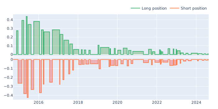
✅ Position views let you analyze your portfolio by focusing on either long or short positions, providing a clear and distinct perspective for each investment strategy.

Separate long and short positions of a basic SMA crossover portfolio

data = vbt.YFData.pull("BTC-USD")
fast_sma = data.run("talib_func:sma", timeperiod=20)
slow_sma = data.run("talib_func:sma", timeperiod=50)
long_entries = fast_sma.vbt.crossed_above(slow_sma)
short_entries = fast_sma.vbt.crossed_below(slow_sma)
pf = vbt.PF.from_signals(
    data,
    long_entries=long_entries,
    short_entries=short_entries,
    fees=0.01,
    fixed_fees=1.0
)

long_pf = pf.long_view
short_pf = pf.short_view

fig = vbt.make_subplots(rows=2, cols=1, shared_xaxes=True, vertical_spacing=0.01)
fig = long_pf.assets.vbt.plot_against(
    0,
    trace_kwargs=dict(name="Long position", line_shape="hv", line_color="mediumseagreen"),
    other_trace_kwargs=dict(visible=False),
    add_trace_kwargs=dict(row=1, col=1),
    fig=fig
)
fig = short_pf.assets.vbt.plot_against(
    0,
    trace_kwargs=dict(name="Short position", line_shape="hv", line_color="coral"),
    other_trace_kwargs=dict(visible=False),
    add_trace_kwargs=dict(row=2, col=1),
    fig=fig
)
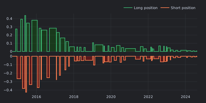
fig.show()

long_pf.sharpe_ratio

0.9185961894435091

short_pf.sharpe_ratio

0.2760864152147919

Index records

New in1.12.0

✅ How can you backtest time- and asset-anchored queries such as "Order X units of asset Y on date Z"? Typically, you would need to build a full array and set each detail manually. Now, there is a simpler way: with preparers and redesigned smart indexing, you can provide all information in a compressed record format! Behind the scenes, the record array is translated into a set of index dictionaries—one for each argument.

Define a basic signal strategy using records

data = vbt.YFData.pull(["BTC-USD", "ETH-USD"], missing_index="drop")
records = [
    dict(date="2022", symbol="BTC-USD", long_entry=True),  
    dict(date="2022", symbol="ETH-USD", short_entry=True),
    dict(row=-1, exit=True),
]
pf = vbt.PF.from_signals(data, records=records)  
pf.orders.readable

   Order Id   Column              Signal Index            Creation Index
0         0  BTC-USD 2022-01-01 00:00:00+00:00 2022-01-01 00:00:00+00:00  \
1         1  BTC-USD 2023-04-25 00:00:00+00:00 2023-04-25 00:00:00+00:00
2         0  ETH-USD 2022-01-01 00:00:00+00:00 2022-01-01 00:00:00+00:00
3         1  ETH-USD 2023-04-25 00:00:00+00:00 2023-04-25 00:00:00+00:00

                 Fill Index      Size         Price  Fees  Side    Type
0 2022-01-01 00:00:00+00:00  0.002097  47686.812500   0.0   Buy  Market  \
1 2023-04-25 00:00:00+00:00  0.002097  27534.675781   0.0  Sell  Market
2 2022-01-01 00:00:00+00:00  0.026527   3769.697021   0.0  Sell  Market
3 2023-04-25 00:00:00+00:00  0.026527   1834.759644   0.0   Buy  Market

  Stop Type
0      None
1      None
2      None
3      None

Portfolio preparers

New in1.12.0

✅ When you pass an argument to a simulation method such as Portfolio.from_signals, it goes through a complex preparation pipeline to convert it into a format suitable for Numba. This pipeline usually involves enum mapping, broadcasting, data type checks, template substitution, and many other steps. To make VBT more transparent, this pipeline has been moved to a separate class, giving you full control over the arguments that reach the Numba functions! You can even extend the preparers to automatically prepare arguments for your own simulators.

Get a prepared argument, modify it, and use in a new simulation

data = vbt.YFData.pull("BTC-USD", end="2017-01")
prep_result = vbt.PF.from_holding(
    data,
    stop_ladder="uniform",
    tp_stop=vbt.Param([
        [0.1, 0.2, 0.3, 0.4, 0.5],
        [0.4, 0.5, 0.6],
    ], keys=["tp_ladder_1", "tp_ladder_2"]),
    return_prep_result=True  
)
prep_result.target_args["tp_stop"]

array([[0.1, 0.4],
       [0.2, 0.5],
       [0.3, 0.6],
       [0.4, nan],
       [0.5, nan]])

new_tp_stop = prep_result.target_args["tp_stop"] + 0.1
new_prep_result = prep_result.replace(target_args=dict(tp_stop=new_tp_stop), nested_=True)  
new_prep_result.target_args["tp_stop"]

array([[0.2, 0.5],
       [0.3, 0.6],
       [0.4, 0.7],
       [0.5, nan],
       [0.6, nan]])

pf = vbt.PF.from_signals(new_prep_result)  
pf.total_return

tp_stop
tp_ladder_1    0.4
tp_ladder_2    0.6
Name: total_return, dtype: float64

sim_out = new_prep_result.target_func(**new_prep_result.target_args)  
pf = vbt.PF(sim_out=sim_out, **new_prep_result.pf_args)
pf.total_return

tp_stop
tp_ladder_1    0.4
tp_ladder_2    0.6
Name: total_return, dtype: float64

Stop laddering

New in1.12.0

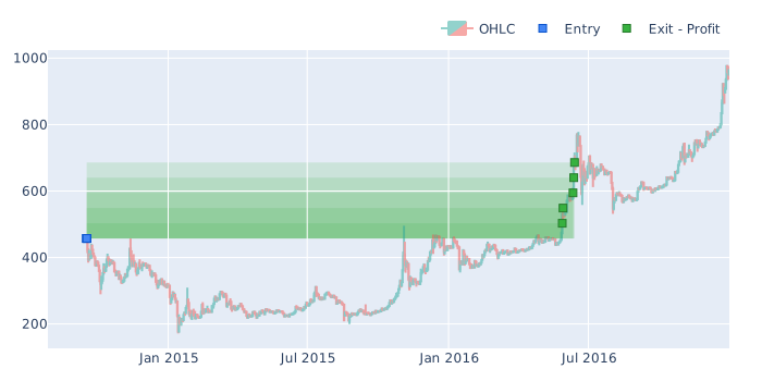
✅ Stop laddering is a technique for incrementally moving out of a position. Instead of providing a single stop value to close a position, you can provide an array of stop values, with each one removing a certain amount of the position when triggered. You can control this amount by choosing a different ladder mode. Thanks to a new broadcasting feature that allows arrays to broadcast along just one axis, the stop values do not need to have the same shape as the data. You can even provide stop arrays of different shapes as parameters!

Test two TP ladders

data = vbt.YFData.pull("BTC-USD", end="2017-01")
pf = vbt.PF.from_holding(
    data,
    stop_ladder="uniform",
    tp_stop=vbt.Param([
        [0.1, 0.2, 0.3, 0.4, 0.5],
        [0.4, 0.5, 0.6],
    ], keys=["tp_ladder_1", "tp_ladder_2"])
)
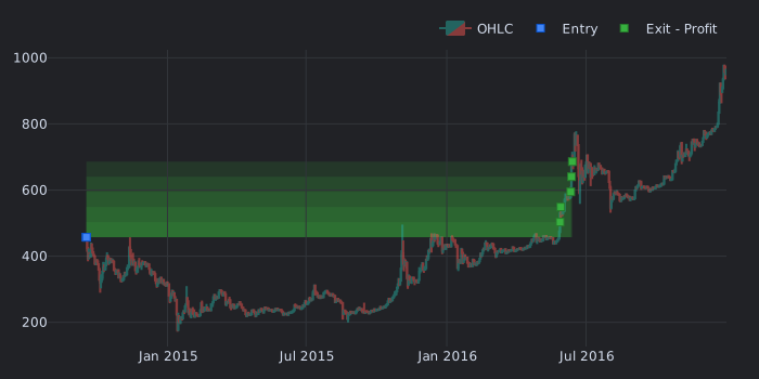
pf.trades.plot(column="tp_ladder_1").show()

Staticization

New in1.11.0

✅ One major limitation of Numba is that functions passed as arguments (that is, callbacks) make the main function uncacheable, forcing it to be recompiled in every new runtime, again and again. This especially affects the performance of simulator functions, as they can take up to a minute to compile. Thankfully, there is a new trick available: "staticization". Here is how it works. First, the source code of a function is annotated with a special syntax. The annotated code is then extracted (also called "cutting" ✂️), modified into a cacheable version by removing any callbacks from the arguments, and saved to a Python file. Once the function is called again, the cacheable version is executed. Sound complicated? Take a look below!

Define the signal function in a Python file, here signal_func_nb.py

from vectorbtpro import *

@njit
def signal_func_nb(ctx, fast_sma, slow_sma):  
    long = vbt.pf_nb.iter_crossed_above_nb(ctx, fast_sma, slow_sma)
    short = vbt.pf_nb.iter_crossed_below_nb(ctx, fast_sma, slow_sma)
    return long, False, short, False

Run a staticized simulation. Running the script again won't re-compile.

data = vbt.YFData.pull("BTC-USD")
pf = vbt.PF.from_signals(
    data,
    signal_func_nb="signal_func_nb.py",  
    signal_args=(vbt.Rep("fast_sma"), vbt.Rep("slow_sma")),
    broadcast_named_args=dict(
        fast_sma=data.run("sma", 20, hide_params=True, unpack=True),
        slow_sma=data.run("sma", 50, hide_params=True, unpack=True)
    ),
    staticized=True  
)

Position info

New in1.11.0

✅ Dynamic signal functions now have access to the current position information, such as (open) P&L.

Enter randomly, exit randomly but only if in profit

@njit
def signal_func_nb(ctx, entries, exits):
    is_entry = vbt.pf_nb.select_nb(ctx, entries)
    is_exit = vbt.pf_nb.select_nb(ctx, exits)
    if is_entry:
        return True, False, False, False
    if is_exit:
        pos_info = ctx.last_pos_info[ctx.col]
        if pos_info["status"] == vbt.pf_enums.TradeStatus.Open:
            if pos_info["pnl"] >= 0:
                return False, True, False, False
    return False, False, False, False

data = vbt.YFData.pull("BTC-USD")
entries, exits = data.run("RANDNX", n=10, seed=42, unpack=True)
pf = vbt.Portfolio.from_signals(
    data,
    signal_func_nb=signal_func_nb,
    signal_args=(vbt.Rep("entries"), vbt.Rep("exits")),
    broadcast_named_args=dict(entries=entries, exits=exits),
    jitted=False  
)
pf.trades.readable[["Entry Index", "Exit Index", "PnL"]]

                Entry Index                Exit Index           PnL
0 2014-11-01 00:00:00+00:00 2016-01-08 00:00:00+00:00     39.134739
1 2016-03-27 00:00:00+00:00 2016-09-07 00:00:00+00:00     61.220063
2 2016-12-24 00:00:00+00:00 2016-12-31 00:00:00+00:00     14.471414
3 2017-03-16 00:00:00+00:00 2017-08-05 00:00:00+00:00    373.492028
4 2017-09-12 00:00:00+00:00 2018-05-05 00:00:00+00:00    815.699284
5 2019-02-15 00:00:00+00:00 2019-11-10 00:00:00+00:00   2107.383227
6 2019-12-04 00:00:00+00:00 2019-12-10 00:00:00+00:00     12.630214
7 2020-07-12 00:00:00+00:00 2021-11-14 00:00:00+00:00  21346.035444
8 2022-01-15 00:00:00+00:00 2023-03-06 00:00:00+00:00 -11925.133817

Time stops

New in1.11.0

✅ Joining other stop orders, time stop orders can close a position either after a certain period of time or on a specific date.

Enter randomly, exit before the end of the month

data = vbt.YFData.pull("BTC-USD", start="2022-01", end="2022-04")
entries = vbt.pd_acc.signals.generate_random(data.symbol_wrapper, n=10, seed=42)
pf = vbt.PF.from_signals(data, entries, dt_stop="M")  
pf.orders.readable[["Fill Index", "Side", "Stop Type"]]

                 Fill Index  Side Stop Type
0 2022-01-19 00:00:00+00:00   Buy      None
1 2022-01-31 00:00:00+00:00  Sell        DT
2 2022-02-25 00:00:00+00:00   Buy      None
3 2022-02-28 00:00:00+00:00  Sell        DT
4 2022-03-11 00:00:00+00:00   Buy      None
5 2022-03-31 00:00:00+00:00  Sell        DT

Target size to signals

New in1.10.0

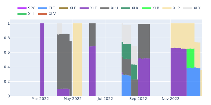
✅ Target size can be converted to signals using a special signal function, giving access to stop and limit order functionality. This is especially useful, for example, in portfolio optimization.

Perform the Mean-Variance Optimization with SL and TP

data = vbt.YFData.pull(
    ["SPY", "TLT", "XLF", "XLE", "XLU", "XLK", "XLB", "XLP", "XLY", "XLI", "XLV"],
    start="2022",
    end="2023",
    missing_index="drop"
)
pfo = vbt.PFO.from_riskfolio(data.returns, every="M")
pf = pfo.simulate(
    data,
    pf_method="from_signals",
    sl_stop=0.05,
    tp_stop=0.1,
    stop_exit_price="close"  
)
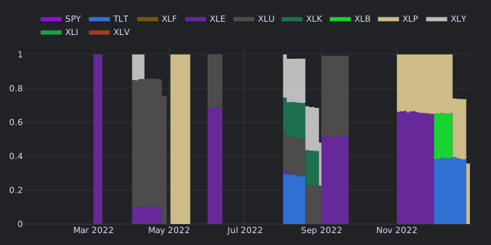
pf.plot_allocations().show()

Target price

New in1.10.0

✅ Limit and stop orders can now be defined using a target price instead of a delta.

Set the SL to the previous low in a random portfolio

data = vbt.YFData.pull("BTC-USD")
pf = vbt.PF.from_random_signals(
    data,
    n=100,
    seed=42,
    sl_stop=data.low.vbt.ago(1),
    delta_format="target"
)
sl_orders = pf.orders.stop_type_sl
signal_index = pf.wrapper.index[sl_orders.signal_idx.values]
hit_index = pf.wrapper.index[sl_orders.idx.values]
hit_after = hit_index - signal_index
hit_after

TimedeltaIndex([ '7 days',  '3 days',  '1 days',  '5 days',  '4 days',
                 '1 days', '28 days',  '1 days',  '1 days',  '1 days',
                 '1 days',  '1 days', '13 days', '10 days',  '5 days',
                 '1 days',  '3 days',  '4 days',  '1 days',  '9 days',
                 '5 days',  '1 days',  '1 days',  '2 days',  '1 days',
                 '1 days',  '1 days',  '3 days',  '1 days',  '1 days',
                 '1 days',  '1 days',  '1 days',  '2 days',  '2 days',
                 '1 days', '12 days',  '3 days',  '1 days',  '1 days',
                 '1 days',  '1 days',  '1 days',  '3 days',  '1 days',
                 '1 days',  '1 days',  '4 days',  '1 days',  '1 days',
                 '2 days',  '6 days', '11 days',  '1 days',  '2 days',
                 '1 days',  '1 days',  '1 days',  '1 days',  '1 days',
                 '4 days', '10 days',  '1 days',  '1 days',  '1 days',
                 '2 days',  '3 days',  '1 days'],
               dtype='timedelta64[ns]', name='Date', freq=None)

Leverage

New in1.9.0

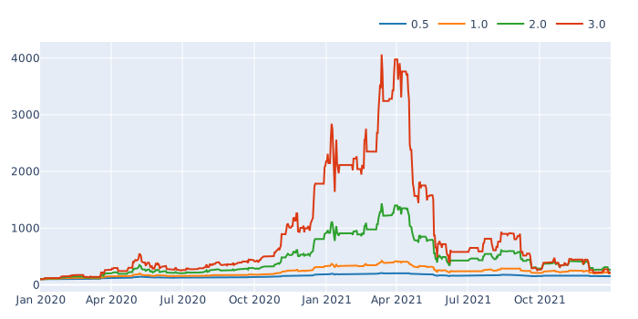
✅ Leverage is now an integral part of portfolio simulation. Supports two leverage modes: lazy (enables leverage only if there is not enough cash) and eager (enables leverage while using only part of the available cash). Allows setting leverage per order, and can also determine the optimal leverage value automatically to fulfill any order requirement! 🏋️

Explore how leverage affects the equity curve in a random portfolio

data = vbt.YFData.pull("BTC-USD", start="2020", end="2022")
pf = vbt.PF.from_random_signals(
    data,
    n=100,
    seed=42,
    leverage=vbt.Param([0.5, 1, 2, 3]),
)
pf.value.vbt.plot().show()

Order delays

New in1.4.1

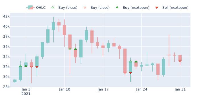
✅ By default, VBT executes every order at the end of the current bar. Previously, if you wanted to delay execution to the next bar, you had to manually shift all order-related arrays by one bar, which made the process error-prone. Now, you can simply specify how many bars in the past should be used to take order information from. In addition, the price argument now supports "nextopen" and "nextclose" as options, providing a one-line solution.

Compare orders without and with a delay in a random portfolio

pf = vbt.PF.from_random_signals(
    vbt.YFData.pull("BTC-USD", start="2021-01", end="2021-02"),
    n=3,
    seed=42,
    price=vbt.Param(["close", "nextopen"])
)
fig = pf.orders["close"].plot(
    buy_trace_kwargs=dict(name="Buy (close)", marker=dict(symbol="triangle-up-open")),
    sell_trace_kwargs=dict(name="Buy (close)", marker=dict(symbol="triangle-down-open"))
)
pf.orders["nextopen"].plot(
    plot_ohlc=False,
    plot_close=False,
    buy_trace_kwargs=dict(name="Buy (nextopen)"),
    sell_trace_kwargs=dict(name="Sell (nextopen)"),
    fig=fig
)
fig.show()

Signal callbacks

New in1.4.0

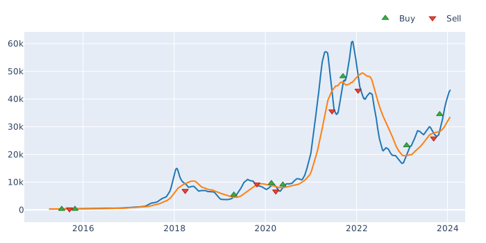
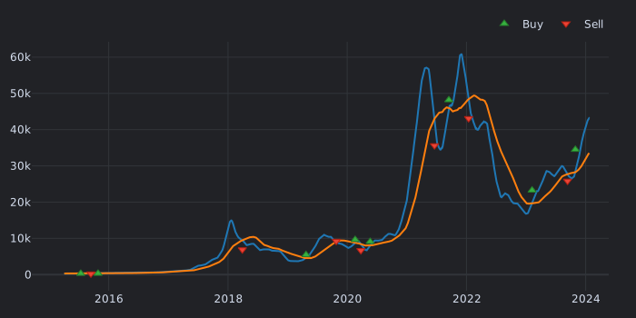
✅ Want to customize your simulation based on signals, or even generate signals dynamically according to the current backtesting environment? Two new callbacks now bring simulator flexibility to the next level: one lets you generate or override signals for each asset at every bar, and another allows you to compute user-defined metrics for the entire group at the end of each bar. Both accept a "context" that contains information about the current simulation state, enabling trading decisions to be made in a way similar to event-driven backtesters.

Backtest SMA crossover iteratively

InOutputs = namedtuple("InOutputs", ["fast_sma", "slow_sma"])

def initialize_in_outputs(target_shape):
    return InOutputs(
        fast_sma=np.full(target_shape, np.nan),
        slow_sma=np.full(target_shape, np.nan)
    )

@njit
def signal_func_nb(ctx, fast_window, slow_window):
    fast_sma = ctx.in_outputs.fast_sma
    slow_sma = ctx.in_outputs.slow_sma
    fast_start_i = ctx.i - fast_window + 1
    slow_start_i = ctx.i - slow_window + 1
    if fast_start_i >= 0 and slow_start_i >= 0:
        fast_sma[ctx.i, ctx.col] = np.nanmean(ctx.close[fast_start_i : ctx.i + 1])
        slow_sma[ctx.i, ctx.col] = np.nanmean(ctx.close[slow_start_i : ctx.i + 1])
        is_entry = vbt.pf_nb.iter_crossed_above_nb(ctx, fast_sma, slow_sma)
        is_exit = vbt.pf_nb.iter_crossed_below_nb(ctx, fast_sma, slow_sma)
        return is_entry, is_exit, False, False
    return False, False, False, False

pf = vbt.PF.from_signals(
    vbt.YFData.pull("BTC-USD"),
    signal_func_nb=signal_func_nb,
    signal_args=(50, 200),
    in_outputs=vbt.RepFunc(initialize_in_outputs),
)
fig = pf.get_in_output("fast_sma").vbt.plot()
pf.get_in_output("slow_sma").vbt.plot(fig=fig)
pf.orders.plot(plot_ohlc=False, plot_close=False, fig=fig)
fig.show()

Limit orders

New in1.4.0

✅ Long-awaited support for limit orders is now available for signal-based simulation! Includes time-in-force (TIF) orders such as DAY, GTC, GTD, LOO, and FOK ⏰ You can also reverse a limit order or create it using a delta for easier testing.

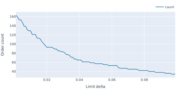
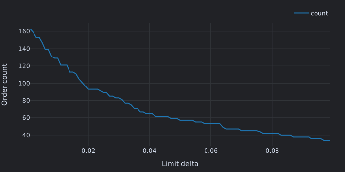
Explore how limit delta affects number of orders in a random portfolio

pf = vbt.PF.from_random_signals(
    vbt.YFData.pull("BTC-USD"),
    n=100,
    seed=42,
    order_type="limit",
    limit_delta=vbt.Param(np.arange(0.001, 0.1, 0.001)),  
)
pf.orders.count().vbt.plot(
    xaxis_title="Limit delta",
    yaxis_title="Order count"
).show()

Delta formats

New in1.4.0

✅ Previously, stop orders could only be provided as percentages. While this worked for single values, it often required extra transformations for arrays. For example, setting SL to ATR meant you needed to know the entry price. More generally, to lock in a specific dollar amount of a trade, you might want to use a fixed price trailing stop. To address this, VBT now offers multiple stop value formats ("delta formats") to choose from.

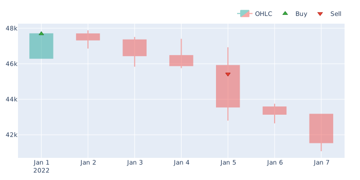
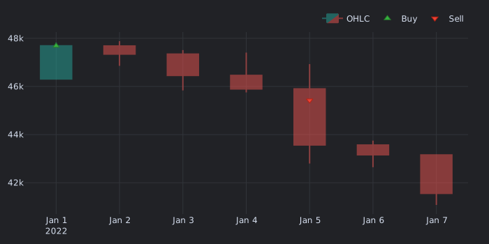
Use ATR as SL

data = vbt.YFData.pull("BTC-USD")
atr = vbt.talib("ATR").run(data.high, data.low, data.close).real
pf = vbt.PF.from_holding(
    data.loc["2022-01-01":"2022-01-07"],
    sl_stop=atr.loc["2022-01-01":"2022-01-07"],
    delta_format="absolute"
)
pf.orders.plot().show()

Bar skipping

New in1.4.0

✅ Simulation based on orders and signals can now (partially) skip bars that do not define any orders, often resulting in significant speedups for strategies with sparsely distributed orders.

Benchmark bar skipping in a buy-and-hold portfolio

data = vbt.BinanceData.pull("BTCUSDT", start="one month ago UTC", timeframe="minute")
size = data.symbol_wrapper.fill(np.nan)
size[0] = np.inf

%%timeit
vbt.PF.from_orders(data, size, ffill_val_price=True)

5.92 ms ± 300 µs per loop (mean ± std. dev. of 7 runs, 1 loop each)

%%timeit
vbt.PF.from_orders(data, size, ffill_val_price=False)

2.75 ms ± 16 µs per loop (mean ± std. dev. of 7 runs, 100 loops each)

Signal contexts

New in1.2.3

✅ Signal generation functions have been redesigned to operate on contexts. This allows you to design more complex signal strategies with less namespace pollution.

Entry at the first bar of the week, exit at the last bar of the week

@njit
def entry_place_func_nb(ctx, index):
    for i in range(ctx.from_i, ctx.to_i):  
        if i == 0:
            return i - ctx.from_i  
        else:
            index_before = index[i - 1]
            index_now = index[i]
            index_next_week = vbt.dt_nb.future_weekday_nb(index_before, 0)
            if index_now >= index_next_week:  
                return i - ctx.from_i
    return -1

@njit
def exit_place_func_nb(ctx, index):
    for i in range(ctx.from_i, ctx.to_i):
        if i == len(index) - 1:
            return i - ctx.from_i
        else:
            index_now = index[i]
            index_after = index[i + 1]
            index_next_week = vbt.dt_nb.future_weekday_nb(index_now, 0)
            if index_after >= index_next_week:  
                return i - ctx.from_i
    return -1

data = vbt.YFData.pull("BTC-USD", start="2020-01-01", end="2020-01-14")
entries, exits = vbt.pd_acc.signals.generate_both(
    data.symbol_wrapper.shape,
    entry_place_func_nb=entry_place_func_nb,
    entry_place_args=(data.index.vbt.to_ns(),),
    exit_place_func_nb=exit_place_func_nb,
    exit_place_args=(data.index.vbt.to_ns(),),
    wrapper=data.symbol_wrapper
)
pd.concat((
    entries.rename("Entries"),
    exits.rename("Exits")
), axis=1).to_period("W")

                       Entries  Exits
Date
2020-01-06/2020-01-12     True  False
2020-01-06/2020-01-12    False  False
2020-01-06/2020-01-12    False  False
2020-01-06/2020-01-12    False  False
2020-01-06/2020-01-12    False  False
2020-01-06/2020-01-12    False  False
2020-01-06/2020-01-12    False   True
2020-01-13/2020-01-19     True  False

Tutorial

Learn more in the Signal development tutorial.

Pre-computation

New in1.0.10

✅ There is a tradeoff between memory usage and execution speed: a dataset with 1000 columns is usually processed much faster than processing a 1-column dataset 1000 times. However, the first dataset also requires 1000 times more memory than the second. That's why, during the simulation phase, VBT primarily generates orders, while other portfolio attributes such as balances, equity, and returns are reconstructed later during the analysis phase if the user needs them. For cases where performance is the main concern, arguments are now available that let you pre-compute these attributes during simulation! ⏩

Benchmark a random portfolio with 1000 columns without and with pre-computation

data = vbt.YFData.pull("BTC-USD")

%%timeit  
for n in range(1000):
    pf = vbt.PF.from_random_signals(data, n=n, seed=42, save_returns=False)
    pf.sharpe_ratio

15 s ± 829 ms per loop (mean ± std. dev. of 7 runs, 1 loop each)

%%timeit
pf = vbt.PF.from_random_signals(data, n=np.arange(1000).tolist(), seed=42, save_returns=False)
pf.sharpe_ratio

855 ms ± 6.26 ms per loop (mean ± std. dev. of 7 runs, 1 loop each)

%%timeit
pf = vbt.PF.from_random_signals(data, n=np.arange(1000).tolist(), seed=42, save_returns=True)
pf.sharpe_ratio

593 ms ± 7.07 ms per loop (mean ± std. dev. of 7 runs, 1 loop each)

Cash deposits

New in1.0.0

✅ Cash can be deposited or withdrawn at any time.

DCA $10 into Bitcoin each month

data = vbt.YFData.pull("BTC-USD")
cash_deposits = data.symbol_wrapper.fill(0.0)
month_start_mask = ~data.index.tz_convert(None).to_period("M").duplicated()
cash_deposits[month_start_mask] = 10
pf = vbt.PF.from_orders(
    data.close,
    init_cash=0,
    cash_deposits=cash_deposits
)

pf.input_value

1020.0

pf.final_value

20674.328828315127

Cash earnings

New in1.0.0

✅ Cash can be continuously earned or spent depending on the current position.

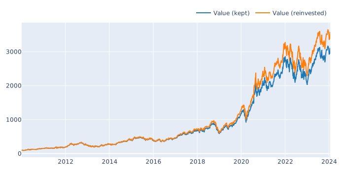
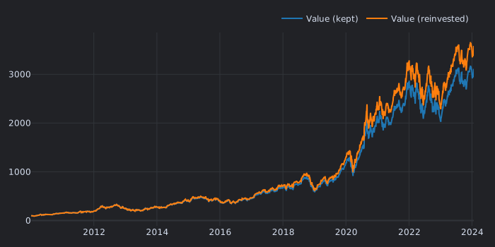
Backtest Apple without and with dividend reinvestment

data = vbt.YFData.pull("AAPL", start="2010")

pf_kept = vbt.PF.from_holding(  
    data.close,
    cash_dividends=data.get("Dividends")
)
pf_kept.cash.iloc[-1]

93.9182408043298

pf_kept.assets.iloc[-1]

15.37212731743495

pf_reinvested = vbt.PF.from_orders(  
    data.close,
    cash_dividends=data.get("Dividends")
)
pf_reinvested.cash.iloc[-1]

0.0

pf_reinvested.assets.iloc[-1]

18.203284859405468

fig = pf_kept.value.rename("Value (kept)").vbt.plot()
pf_reinvested.value.rename("Value (reinvested)").vbt.plot(fig=fig)
fig.show()

In-place outputs

New in1.0.0

✅ The portfolio can now accept and return any user-defined arrays filled during simulation, such as signals. In-place output arrays can broadcast together with regular arrays using templates and broadcastable named arguments. Additionally, VBT will (semi-)automatically determine how to correctly wrap and index each array, for example, whenever you select a column from the entire portfolio.

Track the debt of a random portfolio during the simulation

data = vbt.YFData.pull(["BTC-USD", "ETH-USD"], missing_index="drop")
size = data.symbol_wrapper.fill(np.nan)
np.random.seed(42)
rand_indices = np.random.choice(np.arange(len(size)), 10)
size.iloc[rand_indices[0::2]] = -np.inf
size.iloc[rand_indices[1::2]] = np.inf

@njit
def post_segment_func_nb(ctx):
    for col in range(ctx.from_col, ctx.to_col):
        col_debt = ctx.last_debt[col]
        ctx.in_outputs.debt[ctx.i, col] = col_debt
        if col_debt > ctx.in_outputs.max_debt[col]:
            ctx.in_outputs.max_debt[col] = col_debt

pf = vbt.PF.from_def_order_func(
    data.close,
    size=size,
    post_segment_func_nb=post_segment_func_nb,
    in_outputs=dict(
        debt=vbt.RepEval("np.empty_like(close)"),
        max_debt=vbt.RepEval("np.full(close.shape[1], 0.)")
    )  
)
pf.get_in_output("debt")

symbol                       BTC-USD    ETH-USD
Date
2017-11-09 00:00:00+00:00   0.000000   0.000000
2017-11-10 00:00:00+00:00   0.000000   0.000000
2017-11-11 00:00:00+00:00   0.000000   0.000000
2017-11-12 00:00:00+00:00   0.000000   0.000000
2017-11-13 00:00:00+00:00   0.000000   0.000000
...                              ...        ...
2023-02-08 00:00:00+00:00  43.746892  25.054571
2023-02-09 00:00:00+00:00  43.746892  25.054571
2023-02-10 00:00:00+00:00  43.746892  25.054571
2023-02-11 00:00:00+00:00  43.746892  25.054571
2023-02-12 00:00:00+00:00  43.746892  25.054571

[1922 rows x 2 columns]

pf.get_in_output("max_debt")

symbol
BTC-USD    75.890464
ETH-USD    25.926328
Name: max_debt, dtype: float64

Flexible attributes

New in1.0.0

✅ Portfolio attributes can now be partially or even fully computed from user-defined arrays. This gives you greater control over post-simulation analysis, such as overriding some simulation data, testing hyperparameters without re-simulating the entire portfolio, or avoiding repeated reconstruction when caching is disabled.

Compute the net exposure by caching its components

data = vbt.YFData.pull("BTC-USD")
pf = vbt.PF.from_random_signals(data.close, n=100, seed=42)
value = pf.get_value()  
long_exposure = vbt.PF.get_gross_exposure(  
    asset_value=pf.get_asset_value(direction="longonly"),
    value=value,
    wrapper=pf.wrapper
)
short_exposure = vbt.PF.get_gross_exposure(
    asset_value=pf.get_asset_value(direction="shortonly"),
    value=value,
    wrapper=pf.wrapper
)
del value  
net_exposure = vbt.PF.get_net_exposure(
    long_exposure=long_exposure,
    short_exposure=short_exposure,
    wrapper=pf.wrapper
)
del long_exposure
del short_exposure
net_exposure

Date
2014-09-17 00:00:00+00:00    1.0
2014-09-18 00:00:00+00:00    1.0
2014-09-19 00:00:00+00:00    1.0
2014-09-20 00:00:00+00:00    1.0
2014-09-21 00:00:00+00:00    1.0
                             ...
2023-02-08 00:00:00+00:00    0.0
2023-02-09 00:00:00+00:00    0.0
2023-02-10 00:00:00+00:00    0.0
2023-02-11 00:00:00+00:00    0.0
2023-02-12 00:00:00+00:00    0.0
Freq: D, Length: 3071, dtype: float64

Shortcut properties

New in1.0.0

✅ In-place output arrays can be used to override regular portfolio attributes. The portfolio will automatically pick the pre-computed array and perform all future calculations using this array, avoiding redundant reconstruction.

Modify the returns from within the simulation

data = vbt.YFData.pull("BTC-USD")
size = data.symbol_wrapper.fill(np.nan)
np.random.seed(42)
rand_indices = np.random.choice(np.arange(len(size)), 10)
size.iloc[rand_indices[0::2]] = -np.inf
size.iloc[rand_indices[1::2]] = np.inf

@njit
def post_segment_func_nb(ctx):
    for col in range(ctx.from_col, ctx.to_col):
        return_now = ctx.last_return[col]
        return_now = 0.5 * return_now if return_now > 0 else return_now
        ctx.in_outputs.returns[ctx.i, col] = return_now

pf = vbt.PF.from_def_order_func(
    data.close,
    size=size,
    size_type="targetpercent",
    post_segment_func_nb=post_segment_func_nb,
    in_outputs=dict(
        returns=vbt.RepEval("np.empty_like(close)")
    )
)

pf.returns

Date
2014-09-17 00:00:00+00:00    0.000000
2014-09-18 00:00:00+00:00    0.000000
2014-09-19 00:00:00+00:00    0.000000
2014-09-20 00:00:00+00:00    0.000000
2014-09-21 00:00:00+00:00    0.000000
                                  ...
2023-02-08 00:00:00+00:00   -0.015227
2023-02-09 00:00:00+00:00   -0.053320
2023-02-10 00:00:00+00:00   -0.008439
2023-02-11 00:00:00+00:00    0.005569  << modified
2023-02-12 00:00:00+00:00    0.001849  << modified
Freq: D, Length: 3071, dtype: float64

pf.get_returns()

Date
2014-09-17 00:00:00+00:00    0.000000
2014-09-18 00:00:00+00:00    0.000000
2014-09-19 00:00:00+00:00    0.000000
2014-09-20 00:00:00+00:00    0.000000
2014-09-21 00:00:00+00:00    0.000000
                                  ...
2023-02-08 00:00:00+00:00   -0.015227
2023-02-09 00:00:00+00:00   -0.053320
2023-02-10 00:00:00+00:00   -0.008439
2023-02-11 00:00:00+00:00    0.011138
2023-02-12 00:00:00+00:00    0.003697
Freq: D, Length: 3071, dtype: float64

And many more...

⏩ Look forward to more killer features being added every release!

On this page